Satellite embeddings tested on solar farms in central Massachusetts

GISOwl EngineeringOct 21, 2026Earth observation

Scatter plot of thousands of dots in coloured clusters, with small aerial thumbnails of farm fields, a city grid, a forested river, snowy mountains and a reef lagoon linked to individual clusters — Cover illustration; it does not show data from this article.

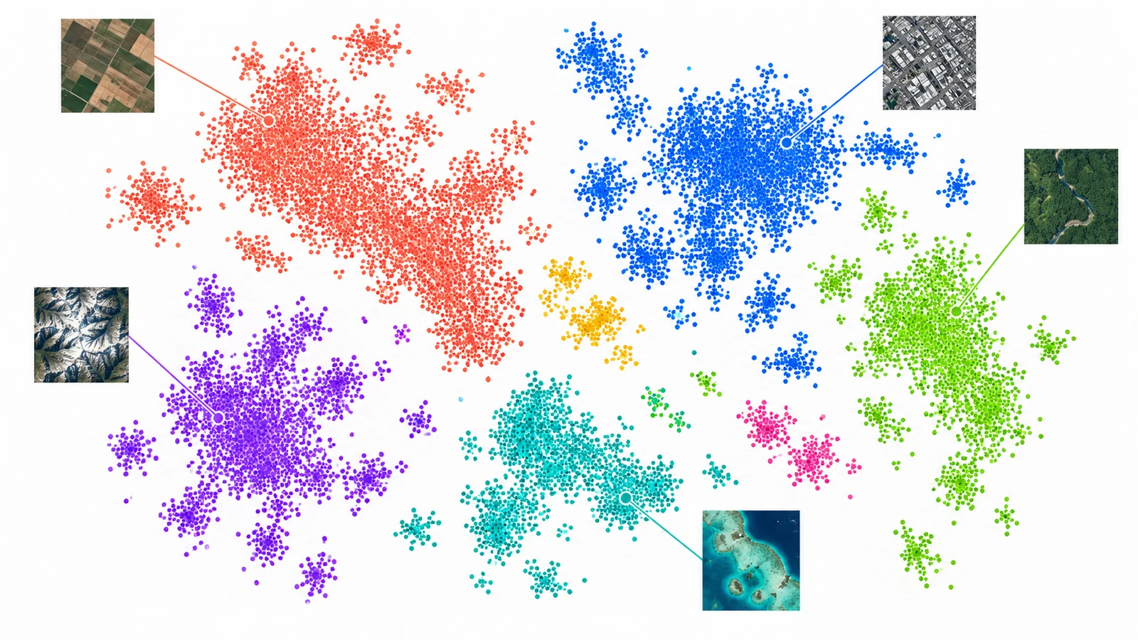
Can Google's Satellite Embedding dataset find "more places like this one", or show what changed between two years, well enough to use without training a model? We tested both on one 20 km square south of Worcester, Massachusetts, with ground-mounted solar farms as the target class. This post covers how to read the data anonymously, the numbers we measured, and the parts we did not get to run.

The short version. Similarity search from five example farms ranked solar pixels more than 200 times better than chance, but results swung a lot depending on which five farms we picked. Change detection between 2018 and 2024 flagged six of nine new farms. It missed three, and new solar made up only a small share of the strongest changes it found.

What the dataset is

The Earth Engine catalog entry describes one 64-dimensional vector per 10 m pixel per year. The bands are A00 to A63, produced by the AlphaEarth Foundations model (Brown et al., 2025). The vectors are unit length, so a dot product is the cosine similarity. The catalog says the embeddings use model v2.1, and that layers have carried DATASET_VERSION 1.1 since 17 November 2025, when the 2017 layer was regenerated. The licence is CC-BY 4.0, with the attribution "The AlphaEarth Foundations Satellite Embedding dataset is produced by Google and Google DeepMind."

The catalog page gives the date range as 2017-01-01 to 2025-01-01. The GCS readme says 2017 through 2025. The mirror index we queried has tiles for every year from 2017 to 2025.

Reading it without Earth Engine credentials

You don't need a Google account. The Source Cooperative mirror, run by Taylor Geospatial Engine, serves the same Cloud-Optimized GeoTIFFs over plain HTTPS at https://data.source.coop/tge-labs/aef/v1/annual/. Its README notes that the copy isn't officially supported by Google. Google's own bucket, gs://alphaearth_foundations, also answered an anonymous HEAD request for its manifest.txt. The readme describes that bucket as "provider pays" as of July 2026. We read all pixel data from Source Cooperative.

The layout, from the readme and confirmed with gdalinfo (GDAL 3.12.4):

Property	Value
Tiling	One directory per year, 120 UTM-zone subdirectories, 8192 × 8192 px tiles
Pixel type	int8, nodata −128, 64 bands, `INTERLEAVE=BAND`, ZSTD, 1024 × 1024 blocks
Compressed block	550 to 770 KB per 1 MB block in the tiles we read
Dequantisation	`sign(v) * (v / 127.5)²`
Orientation	Bottom-up: positive y pixel size, row 0 is the south edge
Index	`aef_index.parquet` / `.gpkg` / `.csv` with UTM and WGS84 bounds per file

Two things cost us time. First, the tiles are stored bottom-up. The mirror ships a warped .vrt next to each tiff to flip them. We read raw windows with pixel offsets and flipped the rows ourselves. Second, a UTM zone boundary is a hard data edge. We read a 128 × 128 window from a 19N tile at the part of the array that lies west of 72°W, and every pixel was −128. A study area that crosses a zone line needs tiles from both zones, in two different CRSs.

The read, with the index entries for 2024 in zone 19N:

import numpy as np
from osgeo import gdal
gdal.UseExceptions()
# env: GDAL_NUM_THREADS=ALL_CPUS GDAL_HTTP_MULTIPLEX=YES GDAL_DISABLE_READDIR_ON_OPEN=EMPTY_DIR
base = "/vsicurl/https://data.source.coop/tge-labs/aef/v1/annual/2024/19N/"
south = gdal.Open(base + "xic18acyygd22iyoi-0000000000-0000008192.tiff")  # y 4587520..4669440
north = gdal.Open(base + "xic18acyygd22iyoi-0000008192-0000008192.tiff")  # y 4669440..4751360
s = south.ReadAsArray(0, 7168, 2048, 1024)[:, ::-1, :]   # raw rows count northwards
n = north.ReadAsArray(0, 0, 2048, 1024)[:, ::-1, :]
q = np.concatenate([n, s], axis=1)                        # (64, 2048, 2048) int8, north-up
lut = np.array([np.sign(v) * (v / 127.5) ** 2 for v in range(-128, 128)], np.float32)
emb = lut[q.astype(np.int16) + 128].reshape(64, -1).T     # (4194304, 64) float32

We aligned the window to the 1024 px block grid, so each year needs exactly 4 blocks per band, 256 in total. On home internet that took 163 s for 2024 and 94 s for 2018. Each north-up int8 GeoTIFF came to 235 MB after ZSTD. Querying the remote GeoParquet index with ogr2ogr -spat took about four minutes. If you plan to do this more than once, download the index.

After dequantisation, vector norms over all 4,194,304 pixels ran from 0.990 to 1.009, with a median of 1.000. That is the unit-length claim, plus int8 rounding.

Study area and reference labels

Box: EPSG:32619, x 254240 to 274720, y 4659200 to 4679680. That is 20.48 km on a side, roughly 71.98°W to 71.72°W and 42.05°N to 42.24°N, covering Charlton, Oxford, Auburn, Leicester and Millbury.
Class: ground-mounted solar. Southern Worcester County has dozens of 1 to 25 ha community-solar farms cut into mixed forest, next to fields, towns, warehouses and the south side of Worcester. That mix gives plenty of confusers.
Labels: the US Large-Scale Solar Photovoltaic Database v4.0 (14 April 2026, 6,611 facilities). It has polygon footprints and an operating year (p_year) from EIA. All 26 facilities in the box are typed greenfield. We rasterised them onto the embedding grid with gdal_rasterize -a case_id -tr 10 10.

USPVDB is better than OpenStreetMap here because it has the build year, but it is still incomplete. It only covers facilities of 1 MW and above, so rooftop arrays, carports and small ground mounts count as "not solar" in every number below. Solar pixels make up about 0.27% of the box. Precision at random is therefore about 0.003.

Similarity search: five farms in, ranked pixels out

Method: pick 5 of the 26 facilities and average every embedding inside their polygons. Renormalise that average to unit length to get the query. Score every pixel with a dot product, drop the query farms' own pixels, and rank the rest. We repeated this for 10 random draws (numpy seed 0), with all 26 farms as eligible positives.

qmask = np.isin(fid, query_ids)
qv = emb[qmask].mean(0); qv /= np.linalg.norm(qv)
score = emb @ qv                 # cosine similarity, 4.2 M pixels
order = np.argsort(-score[~qmask])

Results (P@k is the share of the top k pixels inside a reference polygon; R is the number of remaining positive pixels, about 9,400 to 12,100 depending on the draw):

Draw	P@100	P@1000	P@5000	P@R	Average precision	Farms found (of 21)
0	1.00	0.88	0.79	0.62	0.63	19
1	0.37	0.57	0.57	0.45	0.39	15
2	0.83	0.77	0.68	0.57	0.54	16
3	0.90	0.61	0.58	0.48	0.41	14
4	0.96	0.75	0.60	0.52	0.49	19
5	0.96	0.79	0.75	0.61	0.60	19
6	0.00	0.30	0.54	0.52	0.43	16
7	0.84	0.82	0.71	0.56	0.55	17
8	0.00	0.33	0.51	0.44	0.36	14
9	0.95	0.85	0.73	0.59	0.57	16
Median	0.87	0.76	0.64	0.54	0.52	16

"Found" means at least 25% of a farm's pixels landed in the top R.

Three things stand out.

A plain cosine search with no training gets a median of 76% precision in the top 1,000 pixels, against a 0.3% base rate. On a typical draw it recovers about three quarters of the farms it wasn't shown.
The choice of examples matters more than any other setting. In two draws, all of the top 100 pixels fell outside every reference polygon. Averaging five farms into one vector blurs the class when the farms differ, for example in panel row spacing, ground cover or surrounding forest. A real workflow should keep one query per example and take the maximum score, or fit a small classifier, rather than trusting one averaged vector.
In draw 0, 118 of the top 1,000 pixels were "false" matches. We did not get to inspect them against imagery, so we can't say whether they are unmapped sub-1 MW solar (which would make the true precision higher), rooftops, or something else. For this class the reference gap is real. Any precision figure built on USPVDB alone undercounts.

Change: 2018 against 2024

The catalog says embeddings from different years are consistent enough to compare directly. Per pixel, dot(e2018, e2024) gives a cosine similarity, and low values mean change.

c = np.einsum("ij,ij->i", emb2018, emb2024)

Across the box, the 0.1st, 1st, 5th and 50th percentiles of that dot product were 0.435, 0.748, 0.916 and 0.977. Most of the landscape barely moves. We used the 1st percentile (0.748) as the change threshold.

Solar farms built before the 2018 layer (p_year ≤ 2017, 14 farms) stayed stable. Their per-farm median similarity was between 0.93 and 0.97, and none of their pixels fell below the threshold. That is the result you want: panels in place in both years read as "no change".

The nine farms with p_year from 2019 to 2023 split clearly:

Facility (USPVDB name)	p_year	Pixels	Median dot 2018·2024	Share below 1st pct
Partridge Hill Solar Hybrid	2020	458	0.395	100%
Auburn Solar Project	2022	778	0.452	100%
Oxford Solar	2020	897	0.533	100%
3Colton	2023	483	0.621	76%
Syncarpha Millbury Hybrid (CSG)	2019	1,082	0.626	85%
Cycz Solar Project (CSG) Hybrid	2020	343	0.637	96%
Seaboard Oxford, LLC	2020	316	0.835	1%
Seaboard Charlton, LLC	2020	400	0.865	0%
Millbury MA #1092	2019	185	0.866	0%

Six of nine are obvious. Three are missed outright: their medians sit above 0.83, inside the "barely changed" part of the distribution. We did not check these three against Sentinel-2 imagery from both years, so we don't know why. Two explanations are worth testing. One is that they replaced open fields rather than forest, and a field-to-panels change may move the embedding less than a forest-to-panels change. The other is that the USPVDB polygon or year doesn't match what was on the ground. Until someone looks, this is a hypothesis, not a finding.

The other direction is less flattering. Ranking pixels by lowest similarity, only 5.1% of the 1,000 most-changed pixels and 15.8% of the 4,942 most-changed pixels fell inside new solar farms. (4,942 is the number of new-farm pixels.) In other words, most strong change in this box is something else. The embedding difference flags change of any kind, and in a growing exurban county that means house lots, logging, gravel and whatever else. We didn't classify those pixels, so we can't break them down. To get "where was solar built?" you need both conditions: low 2018·2024 similarity and high 2024 similarity to a solar query.

The baseline we did not finish

The plan was to run the same similarity search on a Sentinel-2 L2A composite from Earth Search (sentinel-2-c1-l2a, MGRS tile 19TBG, which shares the EPSG:32619 10 m grid with the embedding window). The run stopped after screening the 2024 scenes by their scene classification (SCL) layer. Four scenes (12 March, 25 June, 3 and 13 September) were 100% valid in the box. Several others lost 34 to 40% of the box to the swath edge. No reflectance bands were downloaded. So this post has no baseline, and nothing above shows that embeddings beat a simple band-median search on this class. Solar panels are spectrally distinct, being dark in NIR and SWIR against vegetation, so a band median could do well. That comparison is the first thing to run next.

What this does and doesn't show

One class, one landscape, one year pair. The results say nothing about classes that are spectrally ambiguous or that only show up in time series. They also don't tell you whether a query vector built from Massachusetts farms would work in the Mojave or in Brandenburg. We didn't test transfer.
Annual composites hide timing. A farm built in mid-2018 sits partly in the 2018 vector. That's why we left 2018 builds out of the change evaluation. Seasonal effects are folded into each annual vector, so you can't ask "summer only" questions.
Class imbalance shapes the metrics. At a 0.27% base rate, P@k at small k looks great, while average precision of about 0.5 says the tail is noisy. For solar, report facility-level recall alongside pixel precision.
Similarity is not semantics. A high dot product means the model's summary of a pixel's year resembles the query's. Whether that tracks "solar" here depends on the five farms you pick. The Development Seed primer on Earth embeddings makes the same point: embeddings are not labels. Interoperability is still open too. The Cloud-Native Geospatial Forum started sprints in 2026 because embedding datasets have no common format or catalogue metadata yet.

To make this test complete, still to run: the Sentinel-2 baseline on the same 10 draws; a look at the top false matches and the three missed farms in imagery from both years; and an OpenStreetMap overlay to see how many "false" matches are unmapped small solar.

Sources

View as markdown · Edit